1. INTRODUCTION
From the 90s, opening the domestic
market to imported products
and the movement of privatization
promoted by the government, spurred investments in industrial automation
in Brazil to
compete in international industries.
Currently, the need to make the industrial processes more lean
and competitive is
increasingly required due to
globalization. For this reason, the flexibility of manufacturing through
integration with automated systems and devices should
be part of the strategy of industries
who wish to excel in the marketplace.
The Flexible Manufacturing Systems (FMS) are fundamental to face competition from competing
on a global level, the constant technological advances and
ever-changing consumer demand (RAJ et al. 2007). According
to GELENBE and GUENNOUNI (1991), flexible
manufacturing systems are highly
computerized and automated production systems. For these reasons, mathematical programming approaches are very difficult
to solve for very complex system so the simulation of FMS is widely used to
analyze its performance measures (EL-TAMIMI et al. 2011). The advantages of the simulation in manufacturing systems
are also stressed in (JAHANGIRIAN et al. 2010). That article gathered
information from 1997 to 2006 in order to map the coverage as well as the
trends in the area of the simulation of the manufacturing systems.
Another concept extend this definition to production
computer controlled system consisting of several individual machines and workstations, material handling system, system settings and control
system, which can process multiple
items simultaneously in continuous
operation mode for new equipment.
Among these various elements and
devices that make up a flexible manufacturing system, mobile robots for handling materials are a key part of the integration of stations and stages of a production process. The AGV (Automated
Guided Vehicle) consists
in a mobile robots used for
transportation and automatic material
handling, for example for finished
goods, raw materials and products
in process. KRISHNAMURTHY et al. (1993)
point out that the AGV is a driverless vehicle that performs the tasks of handling of flexible materials and is
therefore considered suitable for an FMS environment. Furthermore,
they define a
system of autonomous vehicles (AGVS
- Automated Guided
Vehicle System) "[...] consists of a number
of AGVs operating in a facility, usually controlled by a server" (KRISHNAMURTHY,
1993).
The design and operation
of AGV systems are highly complex due to high levels of randomness and large
number of variables involved. This complexity makes simulation an extremely
useful technique in modeling these systems (NEGAHBAN;SMITH, 2014). For these
reasons several works explore the FMS simulation using AGVs.
From this context, this paper will focus on the use of AGVs technology in an
industry of consumer goods and
the development of a model of virtual
simulation to explore potential
improvements to the system.
The objective of this work is to analyze the use of AGVs integrated into the manufacturing process in
an industry of consumer goods. Furthermore,
the paper proposes to develop a computer simulation
model and validate it through the actual data of the case study, in order to have an additional decision tool to assess possible changes in the process.
In the literature some works deal with the problem of
optimizing the use of AGVs in FMS. In (UM; CHEON; LEE, 2009) a simulation of a
FMS production system using AGVs is presented. The authors, however, do not
possessed real data for the simulation and hypothetic data were used. The
authors stressed the benefits of using the software simulation tools for
achieving a more efficient system.
A different
approach for AGV systems is presented in (JI; XIA, 2010). They considered the
AGV not necessarily as a driverless system, demand quantity
is measured by the unit of weight or volume, buffer storage does not exist in
the system. They have
mentioned the application of its model to the operation of delivery express.
Concerning
about the AGV control problem, (NISHI; ANDO; KONISHI, 2006) presented a
rescheduling procedure can reduce the total
computation time by 39% compared with the conventional method without lowering the
performance level.
A simulation
model of a hypothetical system using AGV which has a job shop environment and
which is based on JIT philosophy was developed in (KESEN; BAYKOÇ, 2007). In
addition, a dispatching algorithm for vehicles moving through stations was
presented in order to improve transportation efficiency.
Several
aspects of AGV systems are discussed at (VIS, 2006). Among them is the design
of the system. It is clear that the design as well as the control system of the
AGV is a difficult task. One important point when designing the system is the
definition of the number of vehicles. In that subject the simulation helps the
designers to take the best decision.
The work presented by (NEGAHBAN; SMITH, 2014) provides a
good review in the simulation of manufacturing systems. An important highlight
is dedicated to the material handling systems where the AGV appears as an
important element. The authors mentioned that the use of the AGVs increases the
productivity in manufacturing systems. However, the design and operation of AGV
systems are highly complex due to high levels of randomness and large number of
variable involved. For these reasons,
the advantages of the computational simulation of the AGV are presented again.
An AGV control system evaluation is proposed in (BERMAN;
SCHECHTMAN; EDAN, 2009). Again, the benefits of the simulation of manufacturing
systems with AGV are presented. The authors used laboratory hardware to
validate the simulation of the control system.
This paper contributes with the subject of simulating AGV
systems when applies real data from a leader of market industry to do both the
investigation of the actual scenario and a simulation of a new proposed
scenario. First results of this work were presented in high level conference
and this paper represents an extended and revised version after the conference
discussions.
2. AGVS – AUTOMATED GUIDED VEHICLES
The AGV has the function
to ensure efficient flow of
materials within the production system. Production systems must be flexible and
must allow the dynamic reconfiguration
of the system. The AGV is a key component
to achieve the objectives of an FMS
(JOSHI and SMITH, 1994). This means that the AGV
should provide the required materials to the appropriate workstation, at the right time and in
the right amount, otherwise the production
system will not perform well, making it less efficient, generating less profit or increasing the operating costs.
In an FMS system, the AGV has the following advantages:
·
Driverless
operation;
·
More efficient
control of the production;
·
Diminishing of the
damages caused by manual material handling;
There are several topologies of AGVs when considering the
positioning system. It can be quoted the inductive system, the magnetic system
and the laser guided system, among others. However, those systems have high
cost and are difficult to maintain according to changes of the environment, and
it can drive only the designated path by sensors which are placed or embedded in.
To overcome those weaknesses, the laser navigation system as a wireless
guidance system has been developed (JUNG et al., 2014).
The factory of the case study of this work uses the laser
guided vehicle (LGV) (FERRARA; GEBENNINI; GRASSI, 2014). The LGV systems have
the advantage of the absence of physical components related to the route. It is
guided by mirrors placed on the walls, as presented in Figure 1.
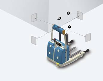
Figure 1:
LGV system
Source:
system-agv
3. CASE STUDY
3.1.
Introduction
The production of toothpastes
is the main focus of the company studied. This product has
the highest profit margin across
the entire range of products manufactured. In addition, it is the market leader in
comparison to the competition. The sector that product creams in the factory has received attention
and investment in
recent years. The aim is to improve the process, guarantying quality and agility in production.
To achieve this goal, the company has focused on modernization of machinery and consequently in increasing
the level of automation of
production. Currently, the sector of toothpastes has 12 production
lines, each one composed of two
main parts: mounting the tube and
filling the tube.
3.2.
Problem definition
Given this context of high performance and commitment to further
increase the level of automation in the factory, the engineering team,
responsible for the continuous improvement of processes, carried out a deep
study to pursue opportunities in the area of toothpaste. Due to the
considerable increase in the volume of production lines, it was identified that
the flow of people, forklifts and other handling equipment also intensified
within a limited space, increasing the likelihood of accidents. Therefore it was necessary to
develop a project that:
a) guarantee organization and security for material handling in an environment with
machines and people;
b) elevate the level of automation in the industry, so that
would result in reduced operating costs.
The characteristics of
this project are discussed in the following. However, currently there
is an additional problem: the
material handling system deployed is already overloaded.
To this issue, this paper refers to the use of simulation to assess possible improvements, which will be discussed in the final stage of the case study.
3.3.
Project features
To reach the expectations of the project, the technology of AGVs
presented itself as an ideal solution to reduce risks within the area of
manufacturing because this type of equipment eliminates the possibility of
human error, compared to use of conventional forklifts. Moreover, the work
environment becomes cleaner, organized flow and generates savings over time
with the reduction of manpower dedicated to material handling.
We
chose the design by the use of LGVs due to its technology capable of providing
flexibility, security and accuracy. There are total six LGVs to date, which are
responsible for two main operations: remove pallets with products from the
lines and take them to the stretch film machine and remove stack of empty
pallets and take them to the production lines. This is presented in Figure 2.
Figure 2: The
route for LGVs
3.4.
developing of the simulation model
For the development of simulations and scenarios
the Promodel® software was
chosen. The Promodel®
software is used to
plan, design and improve new
or current manufacturing processes,
logistics and other systems. It is software that allows building in a simple and visual way,
due to animations, complex logic.
The model was developed in order to simulate the actual situation of the system, which covers the use of LGVs and places where they have
interface points, these being: the centralizing machine pallets, the inputs and outputs of manufacturing lines
and automatic stretch
machine. A CAD picture of the plant was used as background in the Promodel® software. The final model
resulted in the simulation environment as presented in Figure 23. The following will be presented as the model was developed in the Promodel® software.
The model was developed in
order to simulate the actual
situation of the system, which covers
the use of LGVs
and places where they have interface points, these
being: the centralizing machine
pallets, the inputs and outputs of manufacturing lines
and automatic machine
stretch. The following will be presented as the model was developed in the Promodel ® software.
The process begins with the arrival of empty pallets in the central
inventory, where the same are grouped in stacks of 10 and sent to the pallet
centering machine.
From this process, the stacks of pallets are delivered to the 12
production lines using LGV resource. These distributions follow a sequence of
priorities, attending first the lines with higher productivity. After supplying
the lines, the resources are released using the operation
"FREE_LGV1".
After filling the
lines with empty pallets, they are waiting until the arrival of the products (Pallet_LX) with 10 Join rule (join if required)
so that the empty pallets are released one
by one to the stack. With the
arrival of the product (Pallet_LX)
off the line (LX_out) is made the operation of
joining the empty pallet (pallet) with the product by function, "1
PALLET JOIN". After the joint is incremented
one unit in line
with the counter "VAR1
INC, 1" function,
so that the simulation of the counter line show
the number of pieces that come out. They use the "GET
LGV1" function to capture the first available resource, which will hold the drive line out
(LX_out) to the stock
of the stretch machine
(Stretch_X). Is handling
is done with the logic of motion "WAIT 0.5;
MOVE WITH LGV1
then free."
With the arrival of pallet_LX in the stock of the stretch machine, LGV resource
is released and the pallet
is routed to the machine stretch so that it
becomes available. In the pallet machine the
stretch performs the "WAIT
1" operation, which is the time required for to stretch the
pallet and sends it
to the inventory. Again the
function "VAR_stock INC,
1" is used, that is incremented by one unit
in the output total pallet system counter.
With the arrival of pallets in stock, it is forwarded to escape,
leaving the system, thus completing the process.
This process occurs
for the 12 lines simultaneously.
According to information obtained from
the company line 10 has priority over the other lines, so
that the simulation was defined
in the same way.
Based on time-effective
production of each line and the number of finalized pallets in this same period, it was
possible to determine the real-time
release of each pallet per minute for each of the lines.
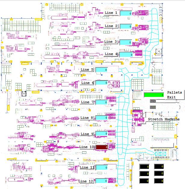
Figure 3:
Promodel® simulation background
From these production data, it was projected two scenarios (which
will be discussed in detail in the
following):
a) Scenario 1 -
Current situation, with 6 LGVs and level of production according to the data collected in 2013 in the company;
b) Scenario 2 –
same parameters as scenario 1, but with
improvements proposed by the authors;
Optionally simulation has added a heating time of 30 minutes. The
heating time is a time of preparation which is not considered in the simulation
results. It was added to the first line supply with empty pallets so that once
production starts, all lines had been already supplied.Você quis dizer: Com a chegada pallets
no estoque, o mesmo é encaminhado para saída (exit), para que saia do sistema,
finalizando assim o processo.
A simulation time of 2160 hours was adopted, which corresponds to 90 days or 3 months of
production. Considering production 24 hours a day, 7 days a week, there
was no need to adopt any stop
or set shifts for the employees.
3.5.
Simulation scenarios
From the simulation model, two different
scenarios were developed for
evaluation of proposals and results,
which will be described below.
3.5.1.
First Scenario: the current production system
The first
scenario is the main subject
of this work. It represents the
current production system. Its main objective is
to evaluate the use of LGVs integrated to the manufacturing
lines and validate the modeling
to compare the results with the actual results of the line. Table 1 presents the resource’s analysis
considering this scenario.
Table
1 – Resource analysis to the first scenario
|
Name
|
Number
Times Used
|
Avg
Time per
Usage(Min)
|
Avg
Time
Travel
to Use
(Min)
|
Avg
Time
Travel
to
Park(Min)
|
%Utilization
|
% In
Use
|
%
Travel
To
Use
|
%Travel
To
Park
|
%
Idle
|
%
Down
|
|
LGV1.1
|
23,689.00
|
4.15
|
1.07
|
1.32
|
95.53
|
75.92
|
19.61
|
0.32
|
0.16
|
4.00
|
|
LGV1.2
|
23,645.00
|
4.16
|
1.07
|
1.40
|
95.52
|
75.95
|
19.57
|
0.34
|
0.16
|
3.99
|
|
LGV1.3
|
23,606.00
|
4.17
|
1.08
|
1.49
|
95.52
|
75.88
|
19.64
|
0.36
|
0.17
|
3.96
|
|
LGV1.4
|
23,668.00
|
4.15
|
1.08
|
1.48
|
95.49
|
75.84
|
19.65
|
0.36
|
0.15
|
4.00
|
|
LGV1.5
|
23,558.00
|
4.18
|
1.08
|
1.40
|
95.55
|
75.98
|
19.57
|
0.33
|
0.15
|
3.97
|
|
LGV1.6
|
23,593.00
|
4.16
|
1.07
|
1.32
|
95.19
|
75.72
|
19.47
|
0.32
|
0.16
|
4.33
|
|
LGVl
|
141,759.00
|
4.16
|
1.07
|
1.40
|
95.47
|
75.88
|
19.58
|
0.34
|
0.16
|
4.04
|
Figure 4 presents a graphical illustration of some
parameters from table 1. In this figure, the last column is the average for the
six AGV.
Figure 4: AGVs: Use, travel time and idle time
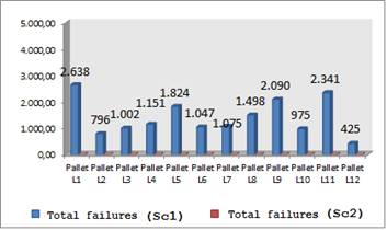
However, despite the high level of use, it can be seen in table 2 failures that occurred in
the system.
Table 2- Entity
Analysis to the first scenario
|
Entity
Name
|
Total failed
|
Total
Exists
|
Current
Qty In System
|
Avg
Time
In
System(Min)
|
Avg
Time In Move Logic (Min)
|
Avg
Time Waiting (Min)
|
Avg
Time in Operation (Min)
|
Avg
Time Blocked (Min)
|
|
PalletL1
|
2,638.00
|
6,424.00
|
0.00
|
23.16
|
3.18
|
16.49
|
1.00
|
2.49
|
|
PalletL2
|
796.00
|
15,202.00
|
2.00
|
10.92
|
2.94
|
4.29
|
1.00
|
2.69
|
|
PalletL3
|
1,002.00
|
14,611.00
|
1.00
|
11.30
|
2.74
|
4.58
|
1.00
|
2.98
|
|
PalletL4
|
1,151.00
|
15,463.00
|
1.00
|
11.21
|
2.55
|
4.61
|
1.00
|
3.06
|
|
PalletL5
|
1,824.00
|
9,250.00
|
2.00
|
15.58
|
2.07
|
9.05
|
1.00
|
3.46
|
|
PalletL6
|
1,047.00
|
10,421.00
|
1.00
|
13.10
|
1.91
|
6.60
|
1.00
|
3.59
|
|
PalletL7
|
1,075.00
|
11,1150.00
|
1.00
|
13.24
|
1.60
|
6.86
|
1.00
|
3.78
|
|
PalletL8
|
1,498.00
|
9,770.00
|
1.00
|
15.97
|
1.33
|
9.54
|
1.00
|
4.10
|
|
PalletL9
|
2,090.00
|
9,080.00
|
2.00
|
19.37
|
1.48
|
12.82
|
1.00
|
4.06
|
|
PalletL10
|
975.00
|
17,806.00
|
1.00
|
7.02
|
1.65
|
2.82
|
1.00
|
1.55
|
|
PalletL11
|
2,341.00
|
8,369.00
|
0.00
|
16.39
|
1.93
|
10.11
|
1.00
|
3.36
|
|
PalletL12
|
425.00
|
1,323.00
|
0.00
|
66.56
|
2.12
|
60.22
|
1.00
|
3.21
|
Figure 5: presents the graphical
information from table 3.
In an attempt to
solve the overload problem in the
use of LGVs, it was added to the model 2 more
unit of LGV, totaling 8 units. Table 3 presents the simulation results with the
increased number of AGVs.
Figure 5: Total failures
Table 3- Resource analysis to the first scenario with 8 LGVs
|
Name
|
Number
Times Used
|
Avg
Time per
Usage(Min)
|
Avg
Time
Travel
to Use
(Min)
|
Avg
Time
Travel
to
Park(Min)
|
%Utilization
|
% In
Use
|
%
Travel
To
Use
|
%Travel
To
Park
|
%
Idle
|
%
Down
|
|
LGV1.1
|
17,715.00
|
5.91
|
1.08
|
1.32
|
95.57
|
80.82
|
14.74
|
0.32
|
0.15
|
3.97
|
|
LGV1.2
|
17,724.00
|
5.90
|
1.08
|
1.39
|
95.56
|
80.75
|
14.82
|
0.33
|
0.16
|
3.95
|
|
LGV1.3
|
17,728.00
|
5.91
|
1.08
|
1.47
|
95.54
|
80.81
|
14.73
|
0.35
|
0.14
|
3.96
|
|
LGV1.4
|
17,708.00
|
5.91
|
1.09
|
1.47
|
95.53
|
80.69
|
14.84
|
0.35
|
0.15
|
3.97
|
|
LGV1.5
|
17,679.00
|
5.93
|
1.08
|
1.40
|
95.56
|
80.85
|
14.71
|
0.33
|
0.14
|
3.96
|
|
LGV1.6
LGV1.7
|
17,827.00
17,810.00
|
5.88
5.88
|
1.07
1.07
|
1.32
1.34
|
95.63
95.53
|
80.87
80.76
|
14.75
14.77
|
0.31
0.32
|
0.15
0.16
|
3.91
3.99
|
|
LGV1.8
|
17,699.00
|
5.92
|
1.08
|
1.34
|
95.55
|
80.86
|
14.69
|
0.32
|
0.15
|
3.98
|
|
LGVl
|
141,890.00
|
5.90
|
1.08
|
1.38
|
95.56
|
80.80
|
14.76
|
0.33
|
0.15
|
3.96
|
Due to the variation in the number of LGVs did
not result in improvement to the
system, the next step was to evaluate the local system. Table 4 presents the
specific data of local single
capacity (Single Location State), and the percentage of sites that feature lock
(Blocked%) and may therefore be contributing to the failures of the system are the inputs of the stretch machine 1, 2 and 3.
The new strategy was the insertion of a buffer into the system. Thus a
new simulation was performed to determining the minimum size of it. The result
is presented in table 5 in the column “maximum contents”.
Table 4: Local single capacity to the first scenario
|
Name
|
Scheduled
Time(HR)
|
% Operation
|
%
Setup
|
%
Idle
|
% Waiting
|
% Blocked
|
% Down
|
|
L1 In
|
2,160.00
|
0.00
|
0.00
|
44.54
|
55.46
|
0.00
|
0.00
|
|
L2 In
|
2,160.00
|
0.00
|
0.00
|
22.00
|
78.00
|
0.00
|
0.00
|
|
L3 In
|
2,160.00
|
0.00
|
0.00
|
22.80
|
77.20
|
0.00
|
0.00
|
|
L4 In
|
2,160.00
|
0.00
|
0.00
|
23.67
|
76.33
|
0.00
|
0.00
|
|
L5 In
|
2,160.00
|
0.00
|
0.00
|
33.02
|
66.98
|
0.00
|
0.00
|
|
L6 In
|
2,160.00
|
0.00
|
0.00
|
25.69
|
74.31
|
0.00
|
0.00
|
|
L7 In
|
2,160.00
|
0.00
|
0.00
|
24.15
|
75.85
|
0.00
|
0.00
|
|
L8 In
|
2,160.00
|
0.00
|
0.00
|
26.50
|
73.50
|
0.00
|
0.00
|
|
L9 In
|
2,160.00
|
0.00
|
0.00
|
25.83
|
74.17
|
0.00
|
0.00
|
|
L10 In
|
2,160.00
|
0.00
|
0.00
|
23.38
|
76.62
|
0.00
|
0.00
|
|
L11 In
|
2,160.00
|
0.00
|
0.00
|
38.01
|
61.99
|
0.00
|
0.00
|
|
L12 In
|
2,160.00
|
0.00
|
0.00
|
40.03
|
59.97
|
0.00
|
0.00
|
|
Pallet Center
|
2,160.00
|
0.00
|
0.00
|
0.00
|
99.06
|
0.94
|
0.00
|
|
Stretch 1
|
2,160.00
|
0.00
|
0.00
|
70.95
|
0.00
|
29.05
|
0.00
|
|
Stretch 2
|
2,160.00
|
0.00
|
0.00
|
70.91
|
0.00
|
28.09
|
0.00
|
|
Stretch 3
|
2,160.00
|
0.00
|
0.00
|
70.10
|
0.00
|
28.90
|
0.00
|
|
Stretch Maq
|
2,160.00
|
99.44
|
0.00
|
0.56
|
0.00
|
0.00
|
0.00
|
Table 5- Buffer
analysis
|
Name
|
Scheduled
Time
(HR)
|
Capacity
|
Total
Entries
|
Avg
Time
Per
Entry(Min)
|
Avg
Contents
|
Maximum
Contents
|
Current
Contents
|
%Utilization
|
|
Locl
|
2,16
|
999,999.00
|
145,739.00
|
7,179.69
|
8,073.77
|
16,150.00
|
16,148.00
|
0.81
|
Once increasing the buffer is not feasible
in this case, another important point to be noted is the operation of the
stretch machine itself. In accordance with table 4, this machine is in
operation in 99.4% of the time, i.e., a potential system bottleneck. At the factory, it can be observed the fact that
frequent queuing of LGVs to unload the pallets in the stretch machine.
Although this work has focused on the use of LGVs,
during the analysis of this scenario and its variations,
it was identified that an improvement
with respect to the stretch machine can result
in gains for the system. Therefore, as an additional contribution to the work, an additional scenario was
developed exploiting the ability of
this machine.
3.5.2.
Second Scenario: improvement of the current production system
As found earlier, the stretch machine represents a possible bottleneck in
the system. Therefore, it was
decided to add a second stretch
machine into the model. With this
change, significant improvement was
observed in the system as presented in table 6.
Table
6: Comparison between first and second scenario: resources
|
Name
|
Avg Time per
Usage(Min)
|
Avg Time
Travel to Use
(Min)
|
%Utilization
|
%
Idle
|
%
Down
|
|
|
Scen1
|
Scen2
|
Scen1
|
Scen2
|
Scen1
|
Scen2
|
Scen1
|
Scen2
|
Scen1
|
Scen2
|
|
LGV1.1
|
4.15
|
2.16
|
1.07
|
1.03
|
95.53
|
69.29
|
0.16
|
27.12
|
4.00
|
3.26
|
|
LGV1.2
|
4.16
|
2.15
|
1.07
|
1.02
|
95.52
|
67.37
|
0.16
|
28.66
|
3.99
|
3.62
|
|
LGV1.3
|
4.17
|
2.15
|
1.08
|
1.02
|
95.52
|
66.28
|
0.17
|
29.72
|
3.96
|
3.63
|
|
LGV1.4
|
4.15
|
2.15
|
1.08
|
1.02
|
95.49
|
64.91
|
0.15
|
31.17
|
4.00
|
3.57
|
|
LGV1.5
|
4.18
|
2.15
|
1.08
|
1.01
|
95.55
|
63.18
|
0.15
|
33.26
|
3.97
|
3.23
|
|
LGV1.6
|
4.16
|
2.14
|
1.07
|
1.00
|
95.19
|
60.78
|
0.16
|
35.26
|
4.33
|
3.63
|
|
LGVl
|
4.16
|
2.15
|
1.07
|
1.02
|
95.47
|
65.30
|
0.16
|
30.86
|
4.04
|
3.49
|
Improvements can also be seen in relation
to the entities and their indicators,
as shown in table 7.
Table
7- Comparison between first and second scenario: entities
|
Entity
Name
|
Total
failed
|
Total Exists
|
Avg Time
In System(Min)
|
Avg Time Waiting (Min)
|
Avg Time Blocked (Min)
|
|
|
Scen1
|
Scen2
|
Scen1
|
Scen2
|
Scen1
|
Scen2
|
Scen1
|
Scen2
|
Scen1
|
Scen2
|
|
PalletL1
|
2,638.00
|
0.00
|
6,424.00
|
9,062.00
|
23.16
|
6.30
|
16.49
|
2.01
|
2.49
|
0.11
|
|
PalletL2
|
796.00
|
0.00
|
15,202.00
|
15,999.00
|
10.92
|
5.86
|
4.29
|
1.83
|
2.69
|
0.10
|
|
PalletL3
|
1,002.00
|
0.00
|
14,611.00
|
15,613.00
|
11.30
|
5.50
|
4.58
|
1.66
|
2.98
|
0.11
|
|
PalletL4
|
1,151.00
|
0.00
|
15,463.00
|
16,614.00
|
11.21
|
5.12
|
4.61
|
1.46
|
3.06
|
0.12
|
|
PalletL5
|
1,824.00
|
0.00
|
9,250.00
|
11,076.00
|
15.58
|
4.22
|
9.05
|
1.07
|
3.46
|
0.10
|
|
PalletL6
|
1,047.00
|
0.00
|
10,421.00
|
11,468.00
|
13.10
|
3.93
|
6.60
|
0.91
|
3.59
|
0.12
|
|
PalletL7
|
1,075.00
|
0.00
|
11,1150.00
|
12,226.00
|
13.24
|
3.47
|
6.86
|
0.75
|
3.78
|
0.12
|
|
PalletL8
|
1,498.00
|
0.00
|
9,770.00
|
11,269.00
|
15.97
|
2.92
|
9.54
|
0.49
|
4.10
|
0.12
|
|
PalletL9
|
2,090.00
|
0.00
|
9,080.00
|
11,172.00
|
19.37
|
3.31
|
12.82
|
0.69
|
4.06
|
0.13
|
|
PalletL10
|
975.00
|
0.00
|
17,806.00
|
18,782.00
|
7.02
|
3.52
|
2.82
|
0.75
|
1.55
|
0.11
|
|
PalletL11
|
2,341.00
|
0.00
|
8,369.00
|
10,710.00
|
16.39
|
4.04
|
10.11
|
1.01
|
3.36
|
0.10
|
|
PalletL12
|
425.00
|
0.00
|
1,323.00
|
1,748.00
|
66.56
|
4.38
|
60.22
|
1.13
|
3.21
|
0.12
|
Figures 6 and 7 presents a comparison of the AGV use
for scenarios 1 and 2 and the total failures for the pallets, respectively.

Figure
6: Comparing AGV use for scenarios 1 and 2
Figure
7: Comparing the pallets total failures for scenarios 1 and 2
4. RESULT ANALYSIS
By analyzing the resources,
as shown in table 1, it can be observed that they are being used to its
maximum capacity within the system
by making use (utilization%)
averaged 95% of the time, with an
average idle (% idle) of while only 0.16%
and not available for operation (down%) of 4%.
In table 2 the failures related to the first scenario was
presented. These failures represent pallets
that were released on the line, but there were no resources available to remove them, i.e., there is an overload of work for LGVs. Additionally,
it is interesting to note that
the line 10, which is currently the
fastest one, is flawed,
however at a lower level than the
majority and the waiting time for
resources is the smallest among all others. Therefore,
it can be concluded that the actual
existing prioritization of this line was correctly
represented by the model.
This overload situation represented in the model validates the simulation because it can be verified in the current reality of the factory. Currently, the lines do
not stop just because the production operators deviate from its main activity, which is monitoring the operation of the line, to
make the removal of pallets
when no LGV is
available to accomplish the task.
This deviation task ends up creating another problem because the operators eventually
leave pallets (empty
or not) blocking the
route of LGVs. When the LGV is faced
with an obstacle, even partially blocking
the way, it stops (as your security configuration) and only return to work when the
obstacle is removed. Consequently, the operation that is already overloaded is
penalized again by
these delays.
Trying to solve the overload problem of the LGVs a new
simulation was carried out considering the insertion of two more AGVs. However, as shown in table 3, it was observed that even with the increased number of LGVs, they remain overloaded and arrival failure continue
to occur in the system.
From the results presented in table 4, a change
in simulation with the addition of
a buffer (Loc1) with the aim of eliminating this block has been made. Initially, the ability of this new buffer was purposely set to
infinity to determine what would be your ideal size. In table
5, the report shows
that the local buffer should be sized for 16,150
pallet positions, which was the maximum amount of entities in this location so that system failures do not occur, or 8,073 positions
that would meet the average and reduce failures arrival,
but did not solve it. However, this design is
impractical.
By comparison of
the results between the first scenario
with the second (Table 6), it can be seen how the
improvements impact the reduction in the
average usage time of LGVs (almost 50%) and reduction
in utilization (30%). This means that the
LGV do not lose more
time in a row to release the
pallet, awaiting availability of the stretch machine.
Improvements related to the entities are also achieved. The
principal was the absence of arrival failures to any
entities. Moreover, the average
waiting times for resource and
lock were drastically reduced. Therefore, the LGVs
are available to
meet all demands and as a consequence there was an increase in the output
system entities, or increase of
production at the same time
interval.
Finally, regarding the use of the additional stretch machine, the operating percentage was
changed from 99.4% to 56.2%, lightening the whole system.
5. CONCLUSIONS
To operate in a global market without barriers and increasingly competitive it is essential to be ready to reduce costs and ensure quality. In this scenario, process automation is becoming a decisive factor for the
success of businesses. Thus, this study contributes to assess
the benefits and impacts to the
automation of material handling
integrated manufacturing lines and propose improvements for the case study through
the use of simulation as
originally defined in the
objectives of this research.
To develop this work, factory visits, interviews with some of the engineers involved in the development and implementation of the project and the current
leader of maintenance, responsible for the operation of LGVs, were performed as
well as a survey of production data. It was finally dedicated a large portion of time to develop a model for computer
simulation to represent satisfactorily
the reality.
The use of simulation proved to be an effective tool to support decision
making. Through it, it can be evaluated different scenarios and possibilities,
helping to define what decision can actually bring more benefits and should be
analyzed more deeply. Finally, through the simulation applied to this case
study it was possible to identify an improvement in the system by adding a
second stretch film machine.
REFERENCES
BERMAN, S.;
SCHECHTMAN, E.; EDAN, Y. (2009) Evaluation of automatic vehicle systems. Robotics and Computer-Integrated
Manufacturing, v. 25, p. 522-528.
EL-TAMIMI, A. M.;
ABIDI, M. H.; MIAN, S. H.; AALAM, J. (2012) Analysis of performance measures of
flexible manufacturing systems. Journal
of King Saud University – Engineering Sciences, v.24, p. 115-129.
FERRARA, A.;
GEBENNINI, E.; GRASSI, A. (2014) Fleet sizing of laser guided vehicles and
pallet shuttles in automated warehouses. International
Journal Production Economics, http://dx.doi.org/10.1016/j.ijpe.2014.06.008.
GELENBE, E.;
GUENNOUNI, H. (1991) Flexism: A flexible manufacturing system simulator. European Journal of Operational Research,
v. 53, p. 149-165.
JAHANGIRIAN, M.;
ELDABI, T.; NASEER, A.; STERGIOULAS, L. K.; YOUNG, T. (2010) Simulation in
manufacturing and business: A review. European
Journal of Operational Research, v. 203, p. 1-13.
JI, M.; XIA, J.
(2010) Analysis of vehicle requirements in a general automated guided vehicle
system based transportation system. Computers
& Industrial Engineering, v. 59, p. 544-551.
JOSHI, S. B.;
SMITH J. S. (1994) Computer Control of Flexible Manufacturing Systems – Research and
Development, Chapman&Hall.
JUNG, K.; KIM,
J.; KIM, J.; JUNG, E.; KIM, S. (2014) Positioning accuracy improvement of laser
navigation using UKF and FIS. Robotics
and Autonomous Systems, v. 62, p. 1241-1247.
KESEN, S. E.; BAYKOÇ,
Ö. F. (2007) Simulation of automated guided vehicle (AGV) systems based on
just-in-time (JIT) philosophy in a job-shop environment. Simulation Modelling Practice and Theory, v. 15, p. 272-284.
KRISHNAMURTHY,
N. N.; BATTA, R.; KARWAN, M. H. (1993) Developing conflict-free routes to
automated guided vehicles. Operation Research
Society of America, v. 41, n. 6,
p. 1077.
NEGAHBAN, A.;
SMITH, J. S. (2014) Simulation for manufacturing system design and operation:
Literature review and analysis. Journal
of Manufacturing Systems, v. 33, p. 241-261.
NISHI, T.; ANDO,
M.; KONISHI, M. (2006) Experimental studies on a local rescheduling procedure
for dynamic routing of autonomous decentralized AGV systems. Robotics and
Computer-Integrated-Manufacturing, v. 22, p. 154-165.
RAJ, T.;
SHANKAR, R.; SUHAIB, M. (2007) A review of some issues and identification of
some barriers in the implementation of FMS. International Journal of
Flexible Manufacturing Systems, v. 19, p. 1-40.
UM, I.; CHEON,
H.; LEE, H. (2009) The simulation design and analysis of a flexible
manufacturing system with automated guided vehicle system. Journal of Manufacturing Systems, v. 28, p. 115-122.
VIS, I. F. A. (2006)
Survey of research in the design and control of automated guided vehicle
systems.
European Journal of
Operational Research, v. 170, p. 677-709.